Measuring working-memory capacity

Working memory (WM) is the name given to the memory system that stores information over short periods, which is strictly limited in terms of duration and capacity. In this post, I present a model for measuring WM capacity from psychophysical data using Bayesian hierarchical inference.

The nature of WM capacity limitation is a source of current debate. Some researchers argue that WM is “slots”-based, stating that we can remember up to a fixed number of discrete items at once (Luck & Vogel, 2013). Others suggest that WM is a finite flexible resource (Ma et al., 2014). Personally, I lean more towards the latter view. However, item-based storage has long been the dominant view, and the maximum number of items stored in WM, denoted by \(k\), remains a popular dependent variable in the cognitive sciences.

A simple way of measuring \(k\) is to apply a formula proposed by either Pashler (1988) or Cowan (2001) to the data from a change-detection task. On each trial, the observer is presented with a stimulus comprising several distinct items (e.g., a visual array of objects) and after a few seconds, a second stimulus is presented. The second stimulus contains at least one item from the original stimulus (the probed item), which may or may not have changed in some way, and the observer indicates whether a change occurred. The choice of formula depends on whether the second stimulus also contains the remaining items from the original stimulus: if so, Pashler’s formula should be used; if it contains just the probed item, Cowan’s should be used.

These formulae are easy to implement and are widely used in research, but there are several problems with them. First, using these formulae, \(k\) can only be calculated from trials with the same set size—experiments typically include trials with various set sizes, so estimates of \(k\) must be calculated separately for each set size and then combined, rather than calculating a single estimate from all the data. Second, since \(k\) can never exceed the set size, it is systematically underestimated whenever the set size is smaller than the true \(k\). Third, the formulae can yield negative values of \(k\), which are obviously impossible. Fourth, the formulae cannot be used to calculate \(k\) at all when performance is at ceiling or floor.

To remedy these issues, Morey (2011) formalized a Bayesian hierarchical model for the measurement of WM capacity from change-detection tasks. The model largely deals with the problems listed above, and is much more efficient (in the sense that it recovers parameters more accurately for a given data set) than Pashler and Cowan’s formulae. Morey provides his own software to fit the model (Morey & Morey, 2011).

I have implemented my own version of this model using PyMC3 (Salvatier et al., 2016). My version is not exactly the same as Morey’s. Most notably, it is much simpler—it measures \(k\) and other model variables just once per observer, and doesn’t consider the potential effects of other factors. I’ll implement a more complex model that estimates such effects in a later post. My model also contains a reparameterization trick to deal with the issue of funneling. The code only applies to the Cowan style of change-detection tasks, although it would be easy to modify it to apply to Pashler-style tasks, or indeed any other variation, provided the decision rule can be specified.

The model

Decision process

We assume that, on a given trial, the observer may or may not suffer a lapse in attention. When a lapse occurs, the observer simply guesses same or different, with no regard for the stimulus. When the observer does not lapse, they perform the task properly. The probability of a non-lapse is denoted by \(z\).

On non-lapse trials, the observer remembers up to \(k\) items from the stimulus. If the set size, \(M\), is less than or equal to \(k\), all of the items are remembered, but if \(M > k\), a random selection of \(k\) items are remembered.

If the probed item was one of the ones remembered, the observer correctly responds same or different, depending on the type of trial. If the probed item was not remembered, the observer guesses, just like on a lapse trial. The probability that the observer guesses different is assumed to be fixed, and is denoted by \(g\).

We have fully defined the decision process. Now we can simulate the observer’s response on a trial, provided we know the set size \(M\), whether the correct response was same or different, and the values of the decision variables, \(z\), \(k\), and \(g\):

def trial(M, different, z, k, g):
    # Returns `True` if different
    from numpy.random import uniform
    if uniform() > z:
        if uniform() < g:
            return True
        else:
            return False
    else:
        if uniform() < k / float(M):
            return different
        else:
            if uniform() < g:
                return True
        else:
            return False

Hits and false alarms

To fit this model to data, we need to define hits and false alarms in a similar way to signal detection theory, and connect them to the variables defined above. We arbitrarily define a hit as a correct response on a different trial, and a false alarm as an incorrect response on a different trial. The observed number of hits, \(H\), follows the probability distribution

where \(h\) is the hit probability, \(D\) is the number of different trials. The corresponding probability distribution for the observed number of false alarms, \(F\), is

where \(f\) is the false-alarm probability and \(S\) is the number of same trials.

The relationships between \(h\) and \(f\), the trial conditions, and the decision parameters defined by these equations:

where

Hierarchical estimation

Suppose that we have data from several observers and we want to estimate \(k\), \(g\), and \(z\) for each of them. It is generally a good idea to do inference on normally distributed variables. However, \(k\) cannot be normal, because negative values of \(k\) are impossible. Similarly, \(g\) and \(z\) cannot be normal either, because they are probabilities and must fall between 0 and 1. Therefore, we apply these transformations:

The new Greek-lettered variables can take any values. Morey (2011) recommends the \(\max\) transformation for \(k\), rather than something like \(\exp\), because 0 is a meaningful value of \(k\).

Next we’ll estimate these parameters hierarchically in order to produce partial pooling, and we’ll use a non-centered parameterization in order to avoid funneling:

where \(i\) indexes the observer, the \(\mu\) and \(\sigma\) variables represent group trends and spread, respectively, and the \(\delta\) variables represent observer-specific standardized offsets.

Priors

All that’s left to do is place priors on the stochastic variables.

Application to real data

Now we will apply this model to the data set provided by Rouder et al. (2008). The following script will download the data, construct the model, sample from its joint posterior, and produce a figure.

import matplotlib.pyplot as plt
import numpy as np
import pandas as pd
import pymc3 as pm
import theano.tensor as tt

from urllib.request import urlopen

from patsy import dmatrix


def main():
    """Download the Rouder et al. (2008) data set, organize it, fit the model, and
    plot the traces.

    """
    # load the data
    a = "https://raw.githubusercontent.com/PerceptionCognitionLab/"
    b = "data0/master/wmPNAS2008/lk2clean.csv"
    df = pd.read_csv(urlopen(a + b), index_col=0)

    # compress into "binomial" format
    data = []
    for (subj, N), _df in df.groupby(["sub", "N"]):

        data.append(
            {
                "subj": subj,
                "M": N,
                "H": _df[_df.ischange.astype(bool)].resp.sum(),
                "D": _df.ischange.sum(),
                "F": _df[(1 - _df.ischange).astype(bool)].resp.sum(),
                "S": (1 - _df.ischange).sum(),
            }
        )
    data = pd.DataFrame(data)
    subjects = data.subj.unique()

    # create a design matrix to map subjects to rows in data
    X = np.asarray(dmatrix("0 + C(subj)", data))

    # create model

    with pm.Model():

        # capacity
        mu = pm.Cauchy(name=r"$\mu_{(\kappa)}$", alpha=0, beta=5)
        de = pm.Normal(name=r"$\delta_{\kappa)}$", mu=0, sigma=1, shape=len(subjects))
        si = pm.HalfCauchy(name=r"$\sigma_{(\kappa)}$", beta=5)
        x = pm.Deterministic(r"$\kappa$", mu + de * si)
        x = pm.Deterministic(r"$k$", tt.largest(x, tt.zeros(len(subjects))))
        k = pm.math.dot(X, x)

        # guesses "same"
        mu = pm.Cauchy(name=r"$\mu_{(\gamma)}$", alpha=0, beta=5)
        de = pm.Normal(name=r"$\delta_{\gamma)}$", mu=0, sigma=1, shape=len(subjects))
        si = pm.HalfCauchy(name=r"$\sigma_{(\gamma)}$", beta=5)
        x = pm.Deterministic(r"$\gamma$", mu + de * si)
        x = pm.Deterministic(r"$g$", pm.math.sigmoid(x))
        g = pm.math.dot(X, x)

        # does not lapse
        mu = pm.Cauchy(name=r"$\mu_{(\zeta)}$", alpha=0, beta=5)
        de = pm.Normal(name=r"$\delta_{\zeta)}$", mu=0, sigma=1, shape=len(subjects))
        si = pm.HalfCauchy(name=r"$\sigma_{(\zeta)}$", beta=5)
        x = pm.Deterministic(r"$\zeta$", mu + de * si)
        x = pm.Deterministic(r"$z$", pm.math.sigmoid(x))
        z = pm.math.dot(X, x)

        # probabilities
        q = tt.smallest(k / data.M, tt.ones(len(data)))
        h = (1 - z) * g + z * q + z * (1 - q) * g
        f = (1 - z) * g + z * (1 - q) * g

        # responses
        pm.Binomial(name="$H$", p=h, n=data.D, observed=data.H)
        pm.Binomial(name="$F$", p=f, n=data.S, observed=data.F)

        # sample and plot
        trace = pm.sample(draws=5000, tune=2000, chains=2)
        pm.traceplot(trace, compact=True)
        plt.savefig("../../assets/images/wm-cap.png", bbox_inches=0, transparent=True)


if __name__ == "__main__":

    main()

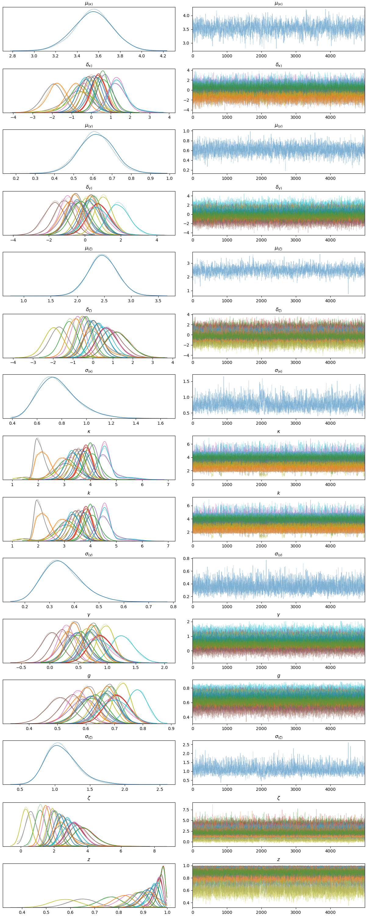Posterior traces under the model.

Next steps

As mentioned above, this model does not allow us to look for factors that might affect \(k\), \(g\), and \(z\), such as different conditions in an experiment, or observer-related effects, such as age. This can be achieved by placing linear models on the group-level parameters. I’ll do this in a future post.

Shameless plug

You can find a real application of this model in one of my papers (Mathias et al., 2018).

References

Cowan, N. (2001). The magical number 4 in short-term memory: A reconsideration of mental storage capacity. Behavioral and Brain Sciences, 24(1), 87–114. 10.1017/S0140525X01003922

Luck, S. J., & Vogel, E. K. (2013). Visual working memory capacity: From psychophysics and neurobiology to individual differences. Trends in Cognitive Sciences, 17(8), 391–400. 10.1016/j.tics.2013.06.006

Ma, W. J., Husain, M., & Bays, P. M. (2014). Changing concepts of working memory. Nature Neuroscience, 17(3), 347–356. 10.1038/nn.3655

Mathias, S. R., Knowles, E. E. M., Barrett, J., Beetham, T., Leach, O., Buccheri, S., Aberizk, K., Blangero, J., Poldrack, R. A., & Glahn, D. C. (2018). Deficits in visual working-memory capacity and general cognition in African Americans with psychosis. Schizophrenia Research, 193, 100–106. 10.1016/j.schres.2017.08.015

Morey, R. D., & Morey, C. C. (2011). WoMMBAT: A user interface for hierarchical Bayesian estimation of working memory capacity. Behavior Research Methods, 43(4), 1044–1065. 10.3758/s13428-011-0114-8

Morey, R. D. (2011). A Bayesian hierarchical model for the measurement of working memory capacity. Journal of Mathematical Psychology, 55(1), 8–24. 10.1016/j.jmp.2010.08.008

Pashler, H. (1988). Familiarity and visual change detection. Perception & Psychophysics, 44(4), 369–378. 10.3758/BF03210419

Rouder, J. N., Morey, R. D., Cowan, N., Zwilling, C. E., Morey, C. C., & Pratte, M. S. (2008). An assessment of fixed-capacity models of visual working memory. Proceedings of the National Academy of Sciences, 105(16), 5975–5979. 10.1073/pnas.0711295105

Salvatier, J., Wiecki, T. V., & Fonnesbeck, C. (2016). Probabilistic programming in Python using PyMC3. PeerJ Comput Science, 2, e55. 10.7717/peerj-cs.55

Version history

• Originally posted March 16, 2020.
• Corrected definition of g on March 27, 2020.

Related posts

• “Bayesian SEM IV: Generalized SEM,” May 19, 2020.
• “Bayesian SEM III: Univariate paramaterization,” May 19, 2020.
• “Bayesian SEM II: Hierarchical latent variables,” May 15, 2020.
• “Bayesian SEM I: Confirmatory factor analysis,” Jan 19, 2020.
• All posts filed under bayesian, cognition, memory, python.